natural experiments

natural experiments
regression discontinuity design
doordash case study
inspired by jessica lachs and matheus facure alves
"hangry" customers 👉 lost customers?
do refunds save customer ltv to some degree?
- a/b testing: unfair to randomly assign refunds
- refund vs. no refund: average lateness differs
confounding!
refund
ltv
min late
"hangry" customers 👉 lost customers?
do refunds save customer ltv to some degree?
- continuity: relationship between ltv and lateness is naturally smooth
- "as good as random": treatment is randomly assigned to near winners and near losers
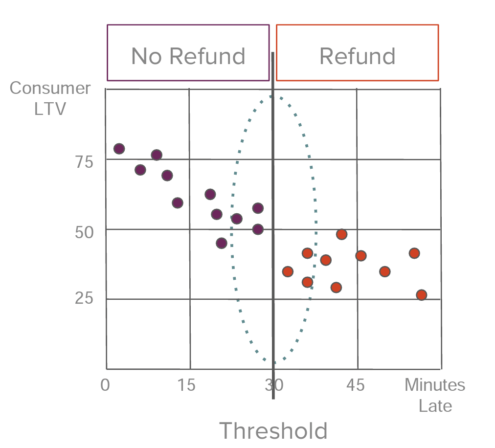
order lateness determines treatment 👉 cutoff: 30 minutes
- "near-loser": 29.9 min late
- "near-winner": 30.1 min late
look for a jump!
"hangry" customers 👉 lost customers?
do refunds save customer ltv to some degree?
running variable: min late
cutoff: 30 min
treatment: 1 - yes; 0 - no
"as good as random"
treated:
intercept at cutoff
intercept at cutoff
treatment effect:
untreated:
interaction: min late may affect ltv differently on each side
def generate_dataset(n, std, b0, b1, b2, b3, lower=0, upper=60, cutoff=30):
    """generate customer LTV under given order lateness and refund status"""

    # generate running variable, treatment status, and errors
    min_late = np.random.uniform(lower, upper, n)
    was_refunded = np.where(min_late < cutoff, 0, 1)
    errors = np.random.normal(0, std, n)

    # use above data to "predict" customer LTV
    ltv = (
        b0
        + b1 * (min_late - cutoff)
        + b2 * was_refunded
        + b3 * (min_late - cutoff) * was_refunded
        + errors
    )

    # return results in a dataframe
    df_late = pd.DataFrame({"min_late": min_late, "ltv": ltv})
    df_late["min_late_centered"] = df_late["min_late"] - cutoff
    df_late["refunded"] = df_late["min_late"].apply(lambda x: 1 if x >= cutoff else 0)

    return df_late

# generate data on 2,000 late orders
df_late = generate_dataset(n=2000, std=10, b0=50, b1=-0.8, b2=10, b3=-0.1)
# DATA PREPARATION
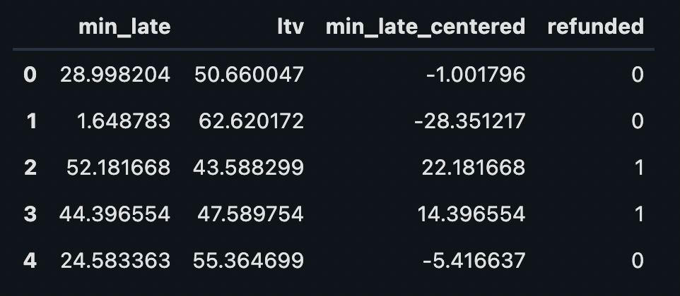
generate toy data
# generate data for 2,000 late orders
df_late = generate_dataset(2000, 10)
df_late.head()
# DATA PREPARATION
generate toy data
modeling
data viz
import statsmodels.formula.api as smf

# fit model
model_all_data = smf.wls("ltv ~ min_late_centered * refunded", df_late).fit()

# model summary
model_all_data.summary().tables[1]
# USING ALL DATA
regress on all data
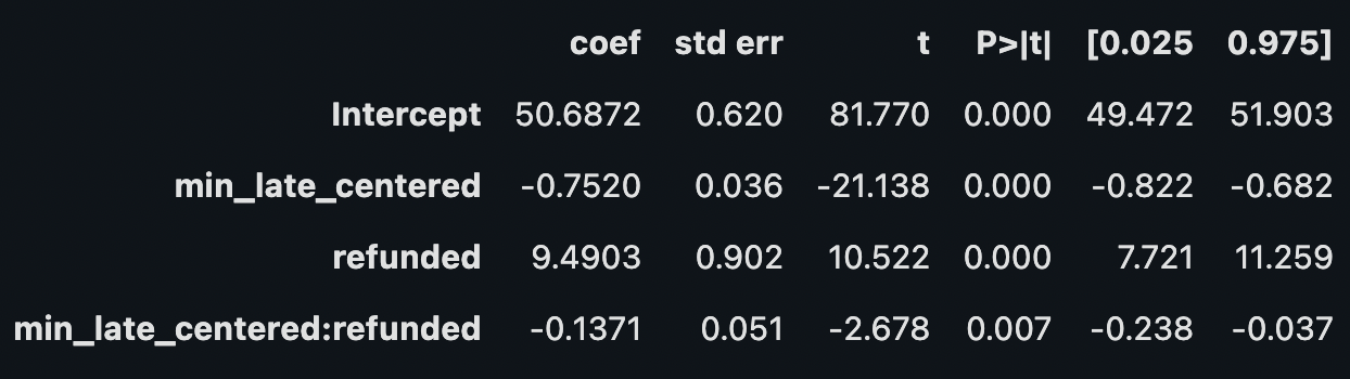
treatment effect: 9.49
# USING ALL DATA
regress on all data
treatment effect: 9.49
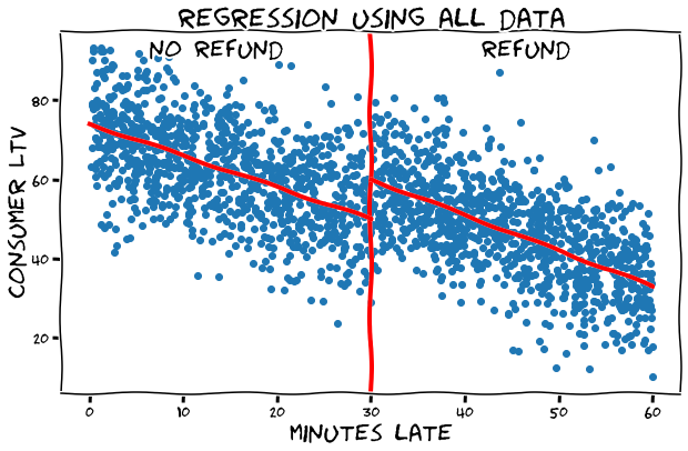
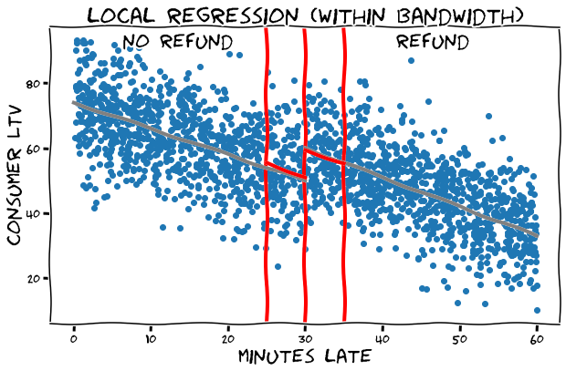
what about just comparing near-losers vs. near-winners?
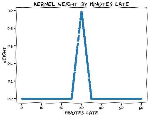
def kernel(min_late, cutoff, bandwidth):
    """assign weight to each data point (0 if outside bandwdith)"""

    # assign weight based on distance to cutoff
    weight = np.where(
        np.abs(min_late - cutoff) <= bandwidth,
        (1 - np.abs(min_late - cutoff) / bandwidth),
        0.0000000001,  # ≈ 0 outside bandwidth (not 0 to avoid division by 0)
    )

    # return weight of each data point
    return weight

df_late["weight"] = df_late["min_late"].apply(lambda x: kernel(x, 30, 5))
# KERNEL WEIGHTING
assign kernel weights to data
- outside bandwidth: not considered
- within bandwidth: closer to cutoff 👉 higher weight
indicates whether point is within bandwidth
# KERNEL WEIGHTING
assign kernel weights to data
# KERNEL WEIGHTING
regress near cutoff
# fit model using weighted data
model_kernel_weight = smf.wls(
    "ltv ~ min_late_centered * refunded",
    df_late,
    weights=df_late["weight"],
).fit()

# model summary
model_kernel_weight.summary().tables[1]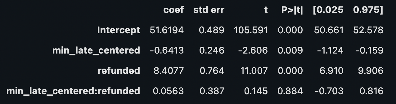
treatment effect: 8.41
# KERNEL WEIGHTING
regress near cutoff
treatment effect: 8.41
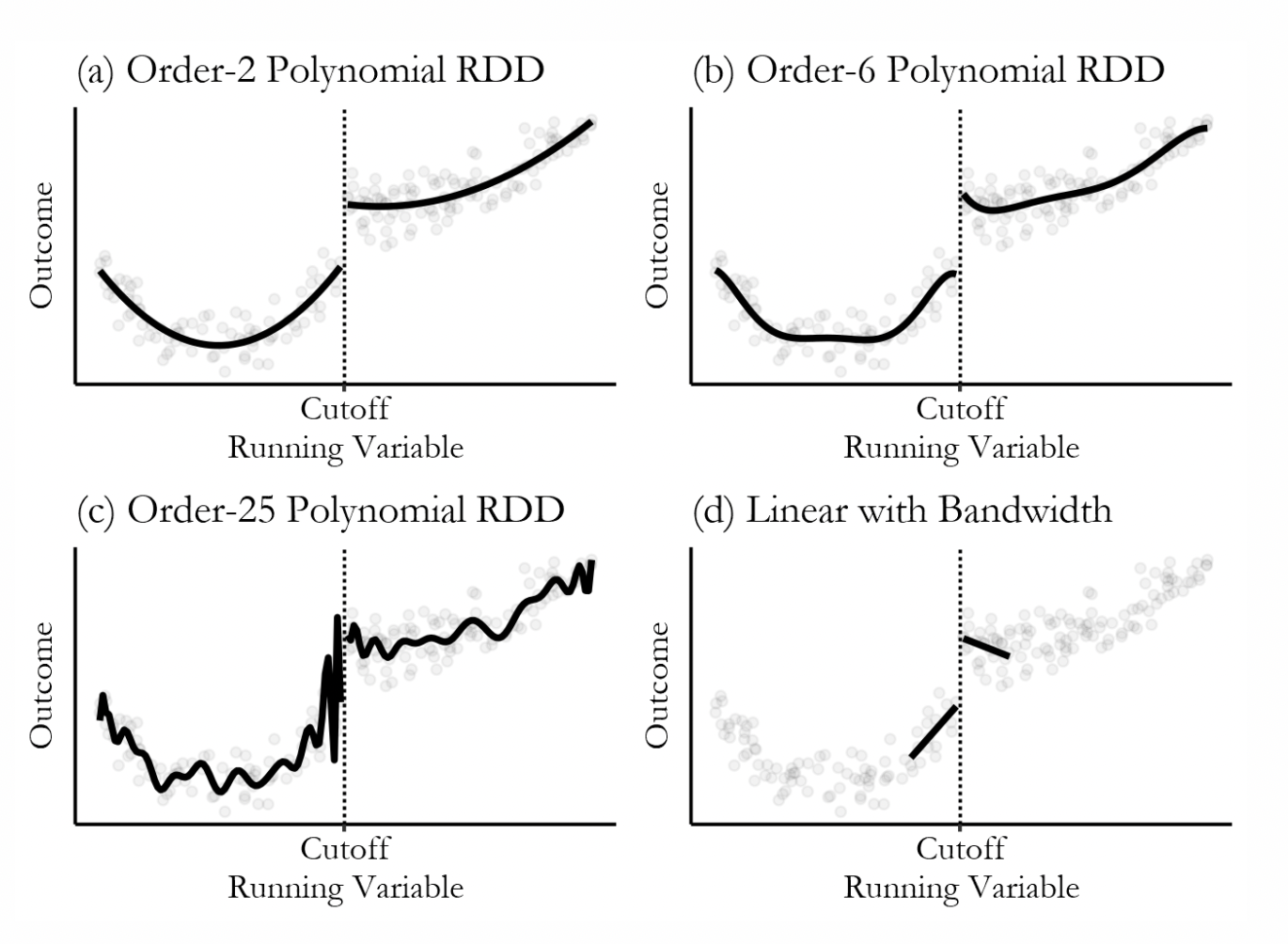
complications of rdd
- optimal bandwidth: use expertise or data-driven methods (cross-validation, imbens & kalyanaraman, 2012)
- not as good as random: e.g., rule-makers manipulate cutoff to include/exclude certain individuals, individuals try to get "mercy pass"
-
fuzziness: "cutoff" impacts the treatment probability but offers no guarantee
- problem: underestimate treatment effect 👉 those below threshold may get treatment and those above may not
- solution: instrumental variables 👉 estimate effect based on actually treated vs. untreated units
- non-linearity: use polynomial regression or local regression (e.g., loess, lowess)
# OTHER NATURAL EXPERIMENTS
veil-of-darkness test
- natural experiment: when daylight saving begins, it gets darker later 👉 7 pm might be dark yesterday but still light today
- outcome: % of black drivers stopped by police at 7 pm increase today? 👉 if so, race may causally impact police stop decisions
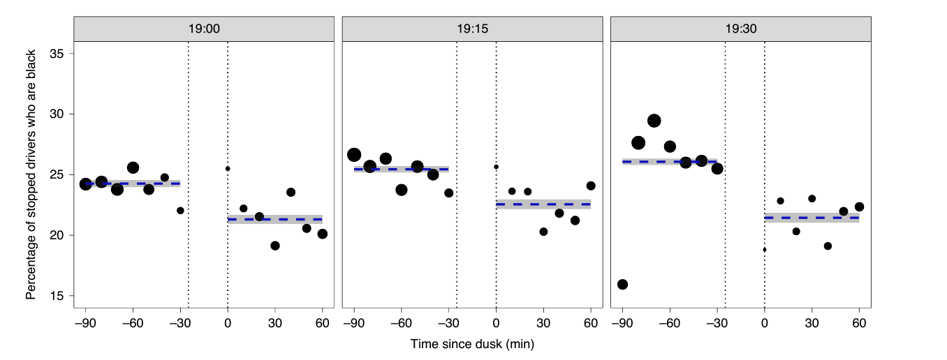
stanford open policing project (pierson et al., 2020)
# OTHER NATURAL EXPERIMENTS
instrumental variables
birth season
schooling
income
confounders
which we can easily find, but don't care about
scale to estimate how treatment affects outcome
1. causally impacts treatment
2. correlated with outcome
3. unrelated to confounders
summary
- why know why: so we can make things happen
- gold standard: randomized controlled trials (a/b testing)
- natural experiments: as good as random, but hard to come by
- statistical control: close "back-door paths"
- counterfactuals: fancier case studies
income
education
intelligence
grades
further resources
books + papers + talks
further resources
an example syllabus...